Part 2: 3D Visualization

3D Projections¶

3D projections allow you to visualize all information from a z-stack in a single view.

1. Open a Z-stack¶

Open one of these sample stacks:

• File > Open Samples > T1 head, or

• File > Open Samples > first instar brain, or

• Use your own z-stack

2. Create a 3D Projection¶

1. Go to Image > Stack > 3D project

2. Try different projection types:

   • Brightest point

   • Nearest point

   • Mean value

What are the differences between these projection types?
What is the effect of checking the Interpolation box?

3. Use the 3D Viewer¶

The 3D Viewer provides interactive volume rendering.

1. Load the instar brain sample again

2. Go to Plugins > 3D viewer

3. Leave all settings as default

4. Click OK

Explore the 3D view by rotating and zooming.

4. Create a Surface Projection¶

1. Open the same image with 3D viewer again

2. Select the Surface option

3. Choose a color to project in

4. Click OK

Advanced 3D Segmentation with TrakEM2¶

TrakEM2 allows you to create subsections and subvolumes for advanced 3D projections.

1. Open T1 Head Sample¶

File > Open Samples > T1-head

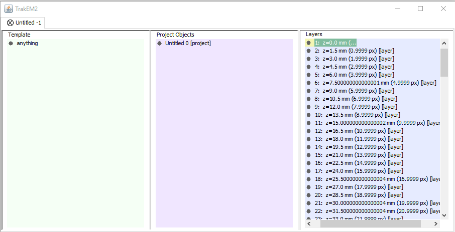
2. Create TrakEM2 Project¶

1. Go to File > New > TrakEM2 (blank)

2. Select a folder for the project to be saved

3. Import the Stack¶

1. Right-click on the black screen

2. Click Import > import stack

3. Select the t1-head image

A new window will open for marking regions in the stack.

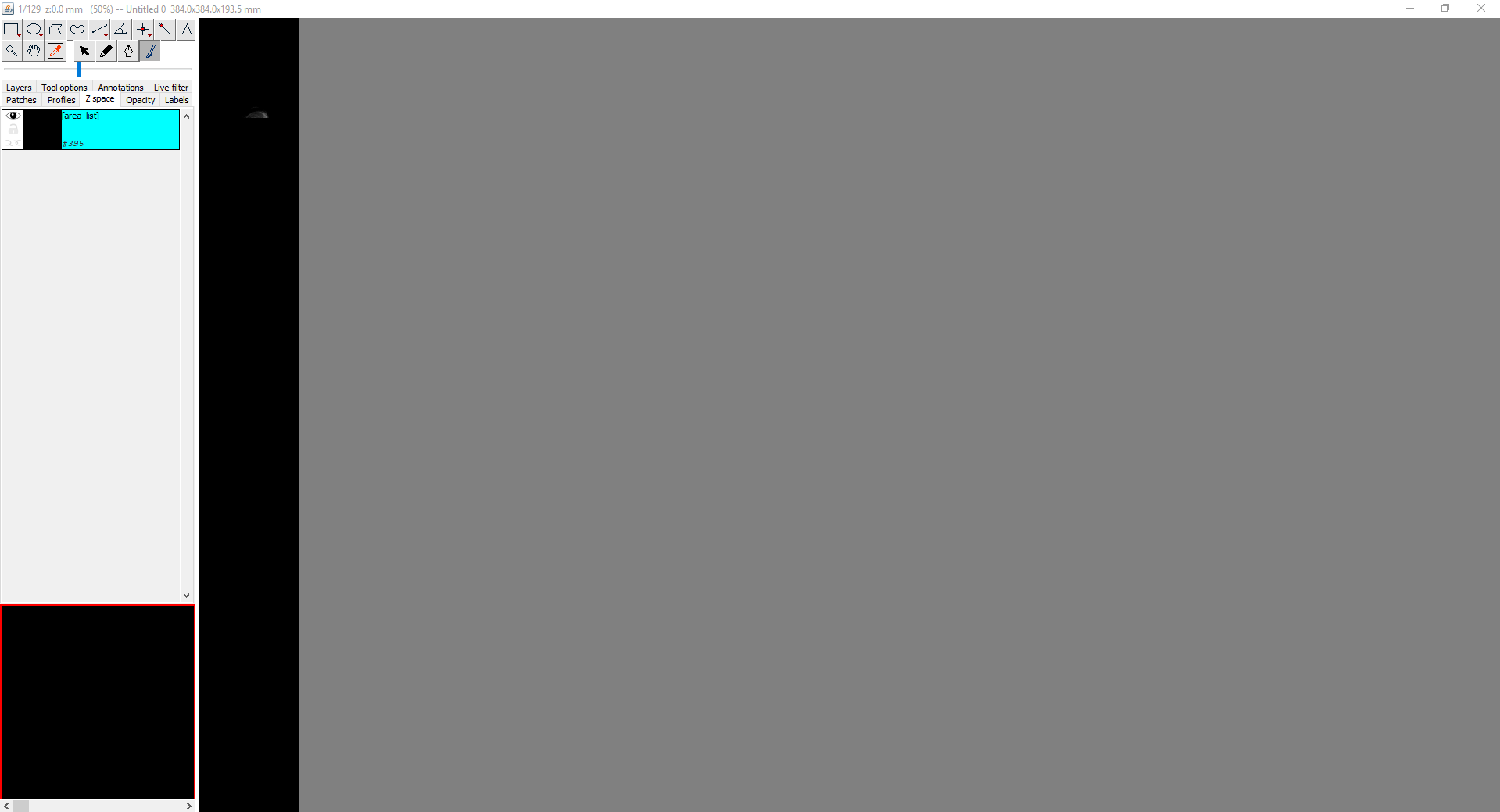
4. Set Up Area List¶

1. Right-click on anything (below template)

2. Select Add new child > area_list

3. Right-click on “untitled” under projects

4. Select Add > new anything

5. Right-click on the new object

6. Select Add > new > area_list

7. Right-click to rename it to “brain”

5. Navigate the Stack¶

In the TrakEM2 window:

• Zoom: Ctrl + scroll wheel

• Navigate slices: Mouse wheel or slider bar

• Pan: Click and drag

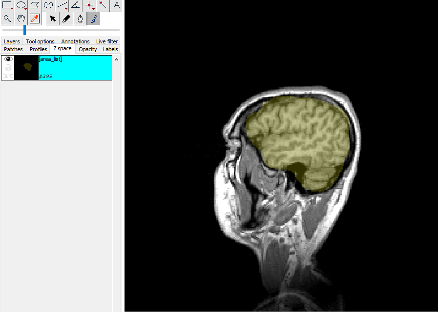
6. Mark the Brain¶

1. Select the first slice where you can see the brain

2. Use the brush tool (automatically selected)

3. Change brush size: Shift + mouse wheel

4. Paint the outline of the brain

5. Remove inaccurate parts: Alt + click

6. Fill holes: Shift + click the middle

7. Mark Multiple Slices¶

1. Move about 10 slices forward

2. Mark the brain again

3. Repeat until you’ve marked the entire brain

4. Make sure the first and last slices are properly marked

8. Interpolate Between Slices¶

Once all slices are marked:

1. Right-click on the image

2. Select Areas > Interpolate all gaps

This fills in all unmarked slices between your annotations.

9. Set Background Color¶

Go to Edit > Options > Colors and set background to black.

10. Export the Segmented Volume¶

1. Right-click on the image

2. Select Export > Image stack under selected area list

This creates a new image with only the brain region.

11. View in 3D¶

1. Go to Plugins > 3D viewer

2. Admire your 3D brain reconstruction

Point Spread Function and Deconvolution¶

Every sub-resolution object in a microscope image is convolved by the microscope’s point spread function (PSF). Deconvolution attempts to mathematically reverse this process.

Understanding PSF¶

The point spread function describes how a single point of light is blurred by the microscope. To perform deconvolution, you need to know the PSF, either by:

• Measuring it with sub-resolution beads, or

• Calculating it theoretically

1. Open Widefield Stack¶

Plugins > LeidenUniv > Teaching > Get widefield stack

2. Generate Theoretical PSF¶

1. Open the PSF Generator: Plugins > LeidenUniv > Teaching > PSF Generator (Born and Wolf)

2. Fill in the appropriate values for GFP:

   • Wavelength: 510 nm

   • Numerical aperture

   • Immersion medium refractive index

   • Pixel size (x, y, z)

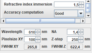
Only change the values in the top block. The other parameters determine the PSF dimensions.

3. Examine the PSF¶

1. Select the PSF image

2. Press Ctrl+Shift+H to see orthogonal views

This displays the intensity distribution from a single sub-resolution object. Notice how one object affects multiple focal planes.

4. Perform Deconvolution¶

Deconvolution is computationally intensive, so work on a small region.

1. Make a selection on the widefield image:

   • Draw a region (~100 × 100 pixels), or

   • Use Edit > Selection > Specify to define exact dimensions

2. Crop or duplicate the selection:

   • Crop: Ctrl+Shift+X or Image > Crop

   • Duplicate: Image > Duplicate (keeps original)

3. Run deconvolution: Plugins > LeidenUniv > Teaching > Iterative deconvolve 3D

4. Select the PSF you generated

5. Wait for the calculation to complete

5. Compare Results¶

Compare the deconvolved image to the original:

• What differences do you observe?

• Are there artifacts introduced by the deconvolution?

• Is the image quality improved?